Category Archives: Technology

Scan Project: Reproducing a Mangaian Toki Through Photogrammetry and 3D Printing

Introduction

This is a project to create a reproduction of a toki adze – a ceremonial axe from Mangaia in the Cook Islands – currently held in the Royal Museums Greenwich archive collection. The toki is approximately 850mm in length, with an intricately carved shaft of repeating cross-cut motifs, a polished dark stone blade, and fine coconut fibre lashing binding blade to haft.
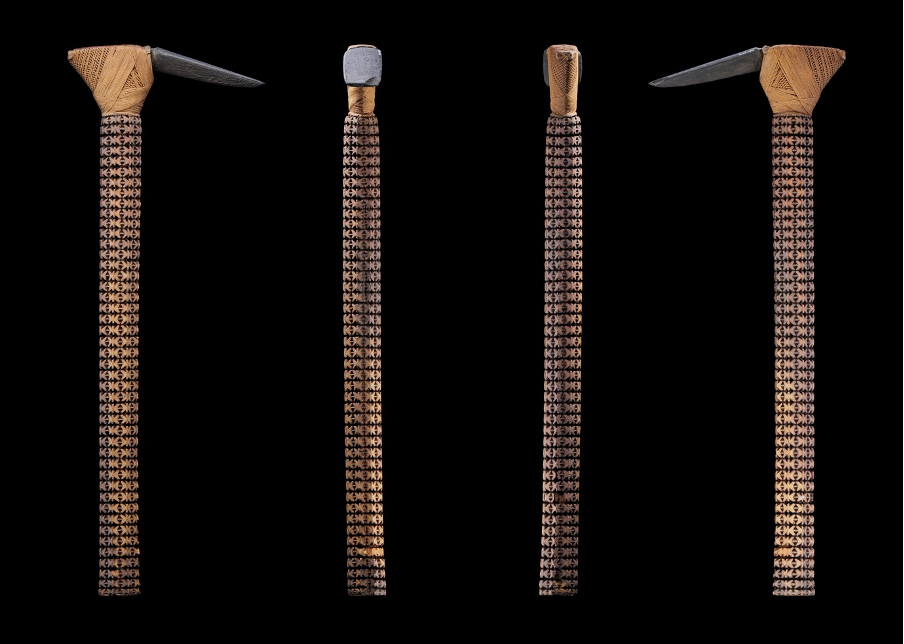
The project sits within maker-identification research into Mangaian toki, undertaken with colleagues at Royal Museums Greenwich and connecting to work by carver Robbie Teremoana Atatoa.

Hundreds of Mangaian toki were removed from the Cook Islands during the nineteenth century and now exist in in museum collections around the world. While preserved physically, they are largely inaccessible to the communities and carving traditions they came from. This project explores whether modern photogrammetry and additive manufacturing can produce a faithful physical reproduction suitable for handling, study and cultural reconnection.

Photogrammetric Capture

This toki was captured over a supervised session in the RMG archive store, working with museum colleagues. Capture setup was tripod / DSLR-based photogrammetry using a Canon EOS R6 Mark III with a 24–105mm lens, shooting RAW at f/8–f/11 with manual focus and image stabilisation off.
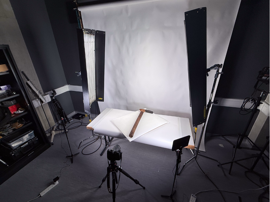
The object sat on protective foam on a turntable, under LED studio lighting. White balance locked in to keep colour consistent across the full image set. The shot strategy was 36 frames per loop (every 10°) across four elevation passes; around 144+ frames for each side side.

Since the toki could not be stood upright – or readily handled – it needed to be photographed and flipped to capture each side separately. This breaks the geometric continuity that photogrammetry relies on, so the two sessions were essentially separate reconstructions from the outset rather than trying to force them into a single alignment.

Reconstruction and the Merge Problem

The image sets were processed with RealityCapture into dense meshes. The two flipped sessions reconstructed very well individually but as separate components – and with a slight scale discrepancy between them of roughly 1.1x – a known issue of turntable photogrammetry where the software has no absolute scale reference.
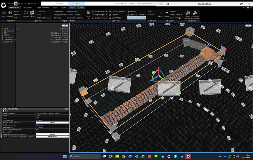
An attempt to resolve the registration externally in CloudCompare didn’t succeed, and the merge was instead worked through inside RealityCapture itself – placing manual control points across features visible in both sessions and iterating until the two halves pulled into agreement. The final alignment was close but not quite perfect – a fraction of residual mismatch that had to be accepted and tidied at the mesh stage rather than eliminated at source.

It’s a real reflection of flip-scan photogrammetry on an object like this: with no shared geometry between the two sessions beyond the object itself, there is a practical limit to how exactly two independent reconstructions can be forced together.

[note for future version: investigate small object laser scanner]

Limitations of Photogrammetric Reconstruction

Photogrammetry captured the overall form and the colour texture very well, but it has known limitations: sharp edges soften and deep dark crevices don’t reconstruct as they’re too much in the dark. On this toki, that meant the deep V-cut channels separating the 45 carved rings along the shaft came through too shallow – one of the most striking features of the object, lost just where the tool marks cut deepest.
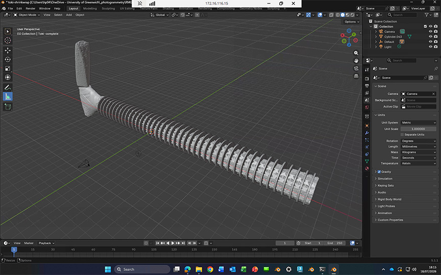
To address this the geometry was brought into Blender 3d modelling software for some digital sculpting to reintroduce features visible on the original but missing from the mesh; sculpt mode sharpening to recover some edge definition and a series of torus rings Boolean subtracted from the shaft to recut those grooves.

This is the point it becomes clear this project has edged from replication / documentation into interpretation – an informed reconstruction rather than a pure scan copy.

Some sculpting back of the lashing zone on the head at this stage too – to make space on the finished print for real cordage, rather than a printed imitation of fibre binding which would never look authentic.

Fabrication

The reproduction was printed on a Bambu Lab H2D. At 850mm the toki far exceeds the 325mm build volume, so the handle was split into three sections in Blender, with the joints planned to fall where they could be disguised within the carved pattern.
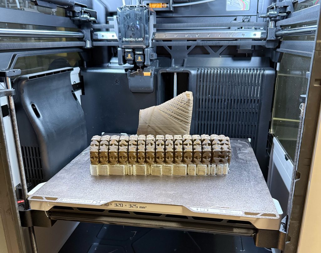
PLA Wood Black Walnut and Rosewood – wood-filled filaments whose matt, slightly fibrous surface takes wood dye convincingly. The head stone was printed separately in a dark technical filament to read as stone against the timber tones of the shaft.

Print orientation took a test print to get right. The instinct was to print the handle sections lying down, but the results read badly: with the shaft on its side, the upper and lower surfaces of the cylinder meet the build plane at very acute angles, so each layer covers a wide sweep of the curve, and the stepping between layers becomes strongly evident – the carving dissolves into visible contour bands. Printed standing up, the geometry meets the layers far better: each ring builds as a series of near-horizontal cross-sections, and the V-cut channels keep more definition. A relatively coarse layer height (0.25–0.28mm) was retained deliberately; layering can work with a wooden object rather than against it.

Assembly

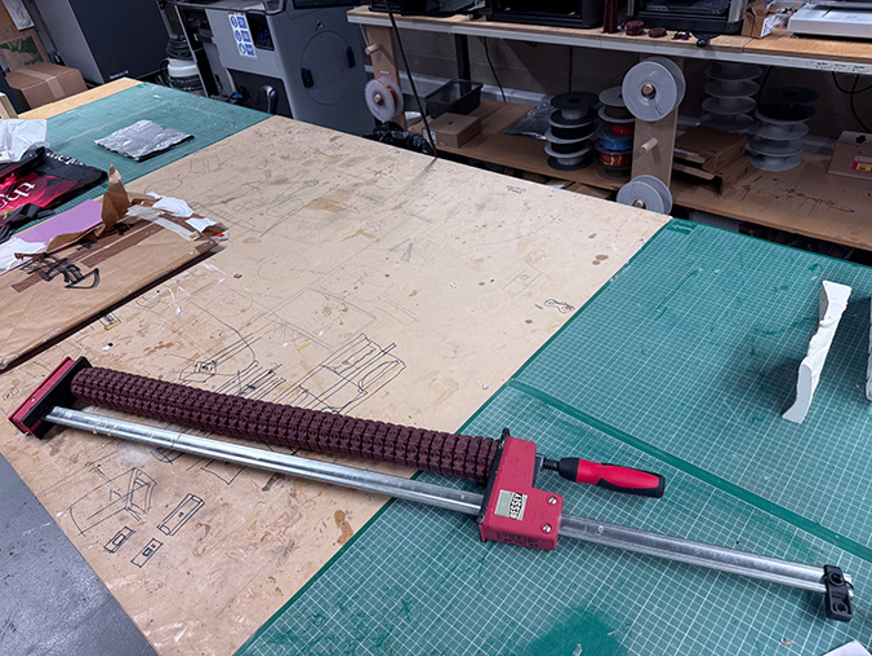
The three handle sections were joined permanently with cyanoacrylate adhesive – glue on one face, activator mist on the other, dry-fitted first, then held firm on contact. CA bonds well to PLA specifically, keying into the layer lines. Glue squeeze-out was kept clear of show surfaces, since cured CA resists dye and telegraphs through wax as a sheen difference.

Assembling before finishing was necessary as the shaft is dyed as one continuous piece, so the tonal gradient – richer and darker toward the head, lighter along the handle can run unbroken across the joints.
Finishing: Building Aged Wood in Layers

The finishing pipeline treats the print as if it were timber, sanding then using actual wood-finishing products rather than just paint effects.

An early lesson: water-based stain beads on smooth PLA. The answer was to work with dyes that penetrate the wood-filled surface – Liberon water-based wood dye as the foundation, with solvent-based spirit dye in a darker oak building depth. The first coat is applied diluted, which runs naturally into the recesses and settles pigment exactly where age would deposit it; subsequent coats build the overall tone.

[note for future version: solvent based dye to darken light coloured filament]
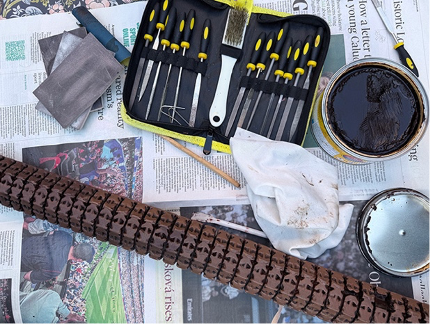
The worn, handled character of the original – lighter peaks where generations of hands have polished the carving – was reproduced by working a nearly-dry cloth of lightened tone (an ochre-tempered mix) across the peaks only, not into the grooves.

The final layer is Liberon Black Bison paste wax in Antique Pine – buffed hard on the peaks for the soft sheen of handled wood, and just lightly into the recesses with a toothbrush so the grooves keep their matt depth.

Lashing

The lashing is where the digital workflow stopped. The coconut fibre binding on the original is not a surface texture but a structural craft in its own right – a specific sequence of wraps and crossings that no 3D printing process can properly replicate. The binding on the reproduction was undertaken by Robbie Teremoana Atatoa, the only member of the project with the skills to do it correctly.

This means the reproduction is not wholly a machine translation of the original: its binding was made by hand, in the proper manner, by a carver whose practice descends directly from the tradition the toki belongs to. Where every other stage of the workflow is a copy of the object, the lashing is a continuation of it.
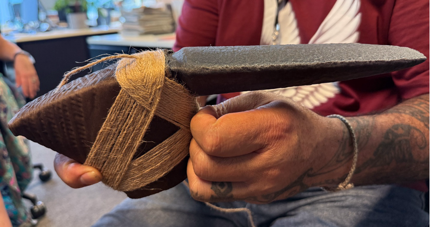
The finished toki is not the original. What it tests is how much of an object’s character – its wear, its tool marks, its accumulated handling – can survive translation through scan data and extruded filament. And unlike many of our reproductions, this one has somewhere to go: it travels with Robbie to New Zealand, a faithful, handleable copy within reach of the carving tradition it came from, while the original remains in the archive in Greenwich.

Credits

  • Scan photography undertaken with access to the original toki kindly facilitated by Royal Museums Greenwich: Ceremonial toki from Mangaia, Cook Islands (ZBA5519).
    Royal Museums Greenwich | Home
  • Equipment for this project was purchased via the ICE Collaborative Research Development Fund 2025/26 
    Institute for Inclusive Communities and Environments
  • Project lead and cultural research: Robbie Atatoa. This recreation was undertaken in support of Robbie’s ongoing work to identify, translate, recreate and revitalise Mangaian toki, developed through his Churchill Fellowship research.
    Robbie Atatoa

POINT CLOUD RENDERING: Blender 3.1

Point clouds may be opened easily enough in Blender but they will not render out unless particular attributes have been assigned to the point cloud using Blender’s Geometry Nodes capability – essentially a real, renderable 3d primitive is located at each point.To import a point cloud the format must be PLY; either export from the point cloud software as PLY or use CloudCompare to open the point cloud and resave as PLY. This may also be a good opportunity to optimise the point cloud file with the CloudCompare Subsample tool – make it smaller; point clouds, particularly from laser scanners, can be very large and will cause performance issues even on high spec machines.

1. In Blender [3.1 or higher] in a new empty file select :

    FILE - IMPORT - Standford (.PLY)

and browse / select the point cloud file

In this example a relatively small file has been imported – this export is from the iPhone Lidar App EveryPoint (Pressing CTL-ALT-Q swaps it to 4 viewports of the point cloud).

If you do not want / do not have colours in your point cloud then you can skip step 2 and go straight to step 3

2. Change to the SHADING tab along the top and click NEW for a new material. Give this a name like PCMaterial.

Now some particular attributes need to be added: from the middle bar click

    ADD - INPUT - ATTRIBUTE

Drop this node to the left and in the name field call it Col – note, must be capital “C”

To the right of this add another node for the colour value:

    ADD - COLOR - HUE SATURATION 

And set the Saturation field to 2.

These nodes can now be linked by dragging from the input / output points. Drag Color to Color and Color to Base Color so the node arrangement looks like this:

3. Switch to the GEOMETRY NODES tab from the top of the screen and click NEW in the middle bar to create a base Group Input and Group Output.

Create 2 new instance nodes (if you drop these on the line they will automatically link up properly)

    ADD - INSTANCE - INSTANCE ON POINTS

and to the right

    ADD - INSTANCE - REALIZE INSTANCES

to end up with this layout:

Next will be another node that will define the real, renderable object that will be at the location of each point in the point cloud – for this example a cube.

    ADD - MESH PRIMITIVE - CUBE

Start with giving the cube the dimensions of 0.01 – these figures will likely need to be altered to fit whatever scale the point cloud is suited for.

Link the Mesh OUT to the Instance IN – but first note the following point:

This is where the point cloud will display as a proper renderable form – BUT it can take a long time depending on size of point cloud. Save first, close other applications, etc.

The rendererable point cloud will now show in the viewport (to speed up this view, or to eliminate viewing errors due to location of the light you can choose to view it as a simple solid form by clicking the solid circle icon, top right hand corner).

The X Y Z dimension of the cube in the cube node can be changed – and the model will update accordingly.

4. Finally the colour (if any) of the point cloud can be brought in by adding another node and linking to the material made in step 2:

    ADD - MATERIAL - SET MATERIAL

Drop this on the Mesh-to-Instance link line and in the bottom field type the name the material was given in the first step “PCMaterial”

Even if there was no colour info in the point cloud this node can be useful for assigning a material to it for colour / shininess / transparency etc.

NOTE: Material operations will only render properly with the Cycles renderer. Eevee render will render much more quickly – but it will be flat colours (which may be fine for mono point clouds).

Credits and thanks to Michael Prostka for YouTube guide and development of PLY import

Point Cloud RENDERING: 3D Studio / V-Ray

It is possible to bring point cloud files into 3D Studio Max and use the software’s advanced camera and animation tools to create rich visualisations of the scans. Do remember that point clouds behave differently to standard 3DS geometry – they cannot be directly manipulated here in the same way as a mesh can; lighting and atmospheric effects will be different – point clouds do not cast shadows, for instance. With point clouds it is more a case of affecting that model rather than manipulating it

Note: standard 3DS will allow you to import the point cloud but it will not render it with the standard 3DS renderer – you will need to set the renderer to V-Ray or Arnold for it to render properly.

IMPORT WITH 3D STUDIO MAX

The following point cloud formats are supported by 3DS:

  • .RCS / .RCP – RCS recommended
  • .LAS / .LAZ
  • .E57
  • .PLY

In 3D Studio go to the Create Geometry panel and select from the drop-down Point Cloud Objects

Then select the Point Cloud button below Object Type and click in the viewport to place roughly where the point cloud is to go – this placeholder will show as a wireframe box.[Note: If this just appears as the 3 red/grey axis lines and not the white box then do a File – Reset and try again; there seems to be a bug sometimes when starting a point cloud]

Below Point Cloud Source click Load Point Cloud and browse to and select your saved RCS file – this will plant the point cloud into the placeholder (it will probably come in huge so you will need to zoom out to see it all)

With the point cloud object selected you will be able to see and edit its properties under the modify tab:

Point Cloud Properties:

  • Limit Box: you can drag the walls of this box to crop the point cloud just to the area you want to be seen – it does not delete the areas outside, just hides them
  • Display Colour Channel Dropdown: choose the colour mode for the points; true colour is their original colour. Single colour allows you to pick one colour for all points, etc.
  • Level of Detail Rendering: for performance related issues you can slide this up and down to get a rougher but quicker representation of the model when you are working on it.
  • Fixed in Rendering: if you click this to On and drag the Level of Detail high then when you render it will render highest quality – and not at the same setting you have for the viewport. [though actually rendering and lower quality levels can create interesting results, so it is worth experimenting with]
  • Point Display: this is the size of the points and the most import variable in changing the look – experimentation here is absolutely key; high figures give fuller (and quicker) renders with a really low figures like 0.1 generate creating nice fine-point results. Note: the point sizes will relate to the resolution of your final render – so what looks fine at 640×480 may be too faint at 1920×1080.
  • Limit Box: this is a way of disabling / enabling the limit box if you have used that to crop your point cloud
  • Display Volumes: this is a useful way to choose only a certain area of the point cloud to be visible by selecting another object such as a cube or sphere to define the extent you want to see. These objects can be combined or inverted.
  • Modifier List: there is a huge list of modifiers available in 3D Studio for bending, twisting, morphing etc. however the vast majority of them will not work on point cloud objects as they are not standard geometry.
True Colour – 1.0 Point size | True Colour – 0.1 Point size | Single Colour – 0.1 Point size
RENDER WITH V-RAY

You must be using the V-Ray renderer (or Arnold) to be able to render point clouds; Scanline, Art, etc. will render blank.

The renders will look much richer than the viewport depictions so it is really worth spending some time getting the point cloud settings right – especially the pixel size which has the most effect.

Full point cloud renders do take time to process but V-Ray has a feature to cap the amount of time it will refine the renders for. This is very useful for experimenting with different settings to get fast feedback. For final renders remove the time limit to allow a full render to be generated.

Render time set to 30 seconds | set to 2 minutes | set to fully complete

In the render setup window – select the V-Ray tab and below Progressive Image Sampler the Render Time field is how long it will spend on the render, so 0.5 will mean the render is processed for 30 seconds, 2 will mean 2 minutes. To allow the render to process entirely enter 0 in this field

Creed Monument – Scan Techniques

The monument of the Creed family sits against the North wall of St. Alfege Church, Greenwich. Sir James Creed (1696 – 1792) was an MP and lead merchant and is buried with his wife at the church. This is a marble monument, about 4 metres high – with markings higher up that suggest a metal cross piece used to be fixed to it.

Photogrammetry Scan

By photographing an object from all sides and capturing many images – with enough overlap so they can be tied together – photogrammetry software can create an accurate 3d model of that object. The resulting mesh object can then be edited and used in CAD / 3D modelling software such as 3DS Max, Rhino, Maya etc. Processes could include replacing textures / materials or applying sun and light models to examine artificial shadow patterns.

This model was created with the software Zephyr Aerial 4.5 using 64 photographs taken with an Apple iPhone X in good daylight. The clarity of a high definition photograph enables the model to carry over very fine, close up detail. Zephyr allows for the mesh to be tidied up, cropped and then exported to the Sketchfab website / service which allows models to be zoomed, spun and examined via browser or app (embedded link below).

Photogrammetry lends itself particularly well to constructing museum-grade scans of smaller, closer objects. It can also deal with larger projects though these are likely require the use of extra equipment – drones, zoom lens, etc. – to obtain distant, high up and otherwise hidden spots to sufficiently cover the entire subject.

Creed Monument: Photogrammetry

Laser Scan

LIDAR technology – radar with light – bounces many light rays off objects within a space to measure distances to those objects and build up a cloud of points with accurate spatial data that represent the shapes found. Typically a tripod mounted laser scanner will rotate the beam vertically and the scanner unit horizontally to capture a 360 sphere of data in a single scan. A number of scans are carried out to best capture the space from all points – and eliminate “blind spots”. These scans are combined together – or registered – to create a single unified point scan.

While the density – and size – of the points can give the impression of solid geometry it is important to remember that this model is floating dots – not solids or meshes that can be edited in the same way as the photogrammetry final output. The size of these points can be adjusted to create revealing, x-ray style views through a building. More practically a point cloud survey of a site can reside as a reference layer on a CAD site plan; the very fine accuracy of a laser scan and the distance it can reach being a distinct advantage.

A Leica BLK360 scanner was used to carry out this scan – with three scans about the monument registering into a single point cloud. Each scan takes around 5 minutes and with so few scans the registration process is straightforward – large projects with lots of scans can be a very involved and time consuming process.

Relative to other laser scanners this model has a range of “only” around 50m (the Faro scanners have nearly three times this). The high concentration of light points sent out also mean that – even with tree coverage around a building or landscape – enough of the beams will still get through to record the semi-hidden project behind.

Creed Monument: Laser Scan

iPhone Polycam App

The Apple iPhone 12 Pro and iPad Pro include a Lidar sensor – a feature to enhance the accuracy of distance and measurement for purposes of augmented reality and camera focusing. This feature has also been utilised by a number of developers to create Lidar scanning apps which open up the opportunity for quick, on-the-go scans straight from the phone.

This app by Polycam is one of the earliest and best to exploit the hardware and point to possibilities of this handset based technique.

This is a lower resolution mesh but the high resolution images wrapped around it still give a good impression of the model. Polycam / Lidar sensor will continuously try to correct itself during the scan sweep to maintain alignment – but there are a few tears in this example where the registration has slipped. More careful movement when scanning would help to prevent this. This scan took about 5 minutes.

Creed Monument – Polycam Scan / iPhone

iPhone TrueDepth Apps

Recent Apple devices use the front facing camera – with “TrueDepth” sensor – to capture 3D information for use with face ID authentication and Animoji. This technique involves projecting 30 000 infrared points and reading back a 3d map of the user’s face. Similar to the Lidar apps, developers have utilised this feature to author apps that can 3d scan with it.

Heges and Capture by Standard Cyborg are two good apps that lever this power of TrueDepth to carry out 3d scans.

Although the capture resolution here is very high the range is short which makes it suitable just for smaller, close-up scans. The other big barrier is that since it uses the front facing camera the handset needs to be pointed at the subject – with the screen away from the viewer. This can make it difficult to see what areas are being scanned – though the Heges app does include a screen share feature where the scan view shows on another device. Constructing a rig that can rotate the camera smoothly all around the model is another option too, where possible, to control speed and shake.